Sorry,,,大概又是比较忙，于是数据分析的内容只好贴上了之前的数理统计的大作业。里面的聚类和回归用的还很不成熟，总之，大家一同学习吧~

PS：里面有很多的代码，不感兴趣的童鞋直接跳过就OK，想做类似的也可以参考。

项目目的

我们对ZOL中关村的手机数据进行分析，希望可以看一看整个手机市场的消费情况，并且对手机产品的改进方向提出一些建议。所以我们下面从两个方面入手。

整个手机消费市场的状况。消费者对于手机性能的关注度。

数据来源

我们爬取了ZOL中关村手机界面上所有在销的商品，这里都是静态网页，非常好爬。具体的数据包含：

商品信息：品牌名称，手机名称，价格。手机参数：主屏尺寸，主屏分辨率，后置摄像头，前置摄像头，电池容量，电池类型，核心数，内存。评论信息：评论人数，评论总分，性价比、性能、续航、外观、拍照评分，评论内容提取。

手机市场的消费状况

手机价格分布描述手机品牌生产产品种类描述手机品牌评论人数分析手机品牌聚类分析

1.1 手机价格分布描述

# import module import pandas as pd import numpy as np import matplotlib.pyplot as plt import seaborn import math from sklearn.cluster import KMeans from mpl_toolkits.mplot3d import Axes3D from wordcloud import WordCloud from PIL import Image from matplotlib import ch ch.set_ch() %matplotlib inline # import data table = pd.read_csv(C:\\Users\\Administrator\\Desktop\\zol_moblie.csv,encoding=gb2312) # plot the distribution of price in total num_bins = 90 fig, ax = plt.subplots(figsize=(9,5)) n, bins, patches = ax.hist(table["price"], num_bins, range = (50,5000)) ax.set_xlabel(Price) ax.set_ylabel(Quatity) ax.set_title(The distribution of price in total) fig.tight_layout() plt.show() # caluculate the basic statistics of price table["price"].describe() # 手机价格的描述 count 2289.000000 mean 1468.736129 std 2100.270967 min 69.000000 25% 599.000000 50% 999.000000 75% 1769.000000 max 50000.000000 Name: price, dtype: float64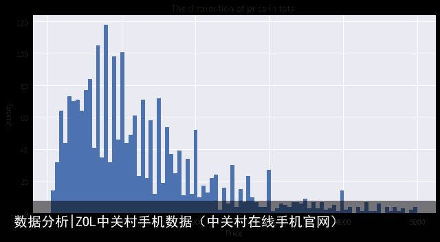可以看出来大多数手机价格都在2000以下，均值在1500左右。商家喜欢设一些1899,2899之类的迷惑性价格。23333~

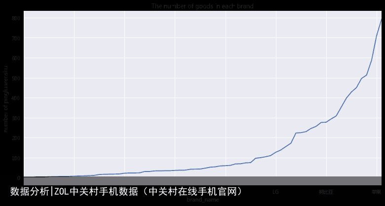
1.2 手机品牌生产产品种类描述¶

table1 = table.iloc[:,[0,2,78]] table1 = table1.drop_duplicates(subset=[good_na]) grouped = table1.groupby(brand_name) table2 = grouped[price].agg(np.count_nonzero) table2 = table2.sort_values(axis=0) fig, ax = plt.subplots(figsize=(13,6.5)) ax.set_xticks(np.linspace(0,70,8)) table2.plot() ax.set_ylabel(number of goods) ax.set_title(The number of goods in each brand) plt.show() print table2[0:40] print table2[40:] brand_name 21克 1 明基 1 汇威 1 独影天幕 1 uphone 1 manta 1 innos 1 VANO 1 小格雷 1 22克 1 23克 1 Ant 1 同洲 2 格力 2 步步高 2 COMIO 2 imoo 2 VEB 3 奇酷 3 8848 4 AGM 4 Google 4 SOYES 4 PPTV 4 蓝魔 4 一加 5 Lovme 5 锤子科技 6 富可视 7 MANN 7 360 8 松下 9 美图 10 乐视 10 SUGAR 11 大神 11 sonim 11 中国移动 11 Microsoft 11 先锋 13 Name: price, dtype: int64 brand_name 乐目 13 Acer 16 HP 16 苹果 17 魅族 21 荣耀 21 小米 25 努比亚 25 神舟 26 华为 29 夏普 30 长虹 30 HTC 36 华硕 41 黑莓 42 vivo 42 酷派 44 TCL 45 LG 47 诺基亚 48 OPPO 48 Moto 48 三星 49 中兴 52 酷比 53 联想 54 索尼 58 康佳 60 朵唯 62 邦华 62 海尔 63 天语 67 纽曼 69 海信 71 飞利浦 78 金立 81 Name: price, dtype: int64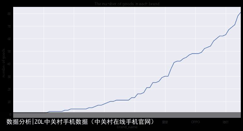我们得到了手机品牌的商品量，苹果有17款，属于比较少的品牌了。最热门的OPPO，vivo，华为之类出产的商品都不是最多的。

1.3 手机品牌评论人数分析

table1 = table[["brand_name","good_na","pinglunrenshu"]] table1 = table1.drop_duplicates(subset=[good_na]) table1 = table1.dropna() # plot the distribution of pinglunrenshu in total num_bins = 90 fig, ax = plt.subplots(figsize=(13,6.5)) n, bins, patches = ax.hist(table1["pinglunrenshu"], num_bins, range = (0,100)) ax.set_xlabel("pinglunrenshu") ax.set_ylabel(Quatity) ax.set_title(The distribution of pinglunrenshu in total) fig.tight_layout() plt.show() table1["pinglunrenshu"].describe() # get the distribution of pinglunrenshu in of each brand grouped = table1.groupby(brand_name) table2 = grouped["pinglunrenshu"].agg(np.mean) table2 = table2.sort_values(axis=0) # plot the distribution of pinglunrenshu in of each brand fig, ax = plt.subplots(figsize=(13,6.5)) ax.set_xticks(np.linspace(0,70,8)) table2.plot() ax.set_ylabel(number of pinglunrenshu) ax.set_title(The number of goods in each brand) plt.show() print table2[0:40] print table2[40:] brand_name 21克 1.000000 Ant 2.000000 COMIO 2.000000 长虹 2.625000 小格雷 3.000000 Acer 3.636364 SOYES 4.500000 22克 5.000000 sonim 5.000000 HP 5.750000 Lovme 6.400000 汇威 8.000000 海尔 8.400000 邦华 9.389831 夏普 10.576923 Google 15.000000 AGM 16.000000 imoo 16.500000 纽曼 17.031250 康佳 17.809524 海信 21.431373 富可视 22.571429 MANN 22.714286 VEB 23.333333 先锋 29.846154 步步高 30.000000 manta 33.000000 酷比 33.510638 黑莓 33.731707 独影天幕 34.000000 PPTV 35.500000 飞利浦 36.476923 蓝魔 36.750000 8848 41.000000 TCL 41.860465 朵唯 42.236364 美图 46.600000 天语 51.607843 中兴 53.368421 酷派 57.928571 Name: pinglunrenshu, dtype: float64 brand_name innos 59.000000 华硕 60.562500 明基 68.000000 同洲 68.500000 中国移动 73.181818 SUGAR 74.272727 乐目 96.363636 Microsoft 99.444444 联想 103.862745 神舟 109.800000 LG 126.409091 格力 137.500000 360 154.875000 Moto 171.354167 索尼 222.824561 金立 224.430380 小米 229.600000 奇酷 245.666667 华为 255.965517 三星 275.530612 努比亚 276.760000 诺基亚 293.270833 HTC 308.571429 锤子科技 353.000000 一加 397.200000 魅族 428.000000 乐视 449.900000 vivo 495.738095 荣耀 512.857143 OPPO 586.208333 苹果 710.529412 大神 793.636364 Name: pinglunrenshu, dtype: float64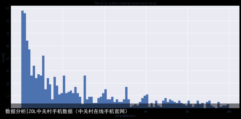评论数量基本和他的销量以及热门程度成正比，我们看到评论最多的手机品牌基本都是我们耳熟能详的。

1.4 手机品牌聚类分析color_dict = {0:red, 1:orange, 2:yellow, 3:green, 4:cyan, 5:blue, 6:yellow} # get the number of types of each brand, the median of brand price, the mean of review number table2 = table.iloc[:,[0,2,78]] table2 = table2.drop_duplicates(subset=[good_na]) grouped = table2.groupby(brand_name) table2 = grouped[price].agg([np.count_nonzero,np.median]) grouped = table.groupby("brand_name") table3 = grouped["pinglunrenshu"].agg([np.mean]) table4 = pd.concat([table2,table3],axis = 1) # fill none with 0 and get the log of data table4["count_nonzero"] = table4["count_nonzero"].map(lambda x: math.log(x)) table4["median"] = table4["median"].map(lambda x: math.log(x)) table4["mean"] = table4["mean"].map(lambda x: math.log(x)) table4 = table4.fillna(0) # cluster all data kmeans = KMeans(n_clusters=4, random_state=0).fit(table4.values) table4[kind] = kmeans.labels_ table5 = table4[kind] # get the label of data la = kmeans.labels_ # plot the result of cluster fig = plt.figure(figsize=(12,7)) ax = fig.add_subplot(111, projection=3d) xs = table4["count_nonzero"].values ys = table4["median"].values zs = table4["mean"].values for i in range(len(xs)): ax.scatter(xs[i], ys[i], zs[i], c=color_dict[la[i]]) for i in kmeans.cluster_centers_: ax.scatter(i[0], i[1], i[2], c=k) ax.set_xlabel(good_kind) ax.set_ylabel(median_) ax.set_zlabel(mean) ax.set_title(The cluster of brand) plt.show() print table5.sort_values()[0:32] print table5.sort_values()[32:] brand_name 独影天幕 0 imoo 0 innos 0 PPTV 0 美图 0 蓝魔 0 manta 0 MANN 0 奇酷 0 步步高 0 VEB 0 格力 0 明基 0 AGM 0 8848 0 富可视 0 同洲 0 Google 0 uphone 1 sonim 1 松下 1 小格雷 1 汇威 1 21克 1 COMIO 1 SOYES 1 22克 1 Lovme 1 23克 1 Acer 1 VANO 1 Ant 1 Name: kind, dtype: int32 brand_name 飞利浦 2 康佳 2 朵唯 2 纽曼 2 酷派 2 海信 2 海尔 2 酷比 2 邦华 2 长虹 2 天语 2 黑莓 2 夏普 2 HP 2 TCL 2 先锋 2 中兴 2 苹果 3 荣耀 3 Moto 3 诺基亚 3 Microsoft 3 LG 3 HTC 3 金立 3 锤子科技 3 360 3 联想 3 OPPO 3 索尼 3 大神 3 神舟 3 vivo 3 一加 3 三星 3 中国移动 3 乐目 3 乐视 3 魅族 3 小米 3 华为 3 华硕 3 SUGAR 3 努比亚 3 Name: kind, dtype: int32

2. 消费者对于手机每一种性能的关注度¶

评论云图性能评分与总评分的回归

2.1 评论云图

table1 = table.iloc[:,18:76] table2 = np.append(table1.iloc[:,0:2].values, table1.iloc[:,2:4].values, axis = 0) for i in range(13): table2 = np.append(table2, table1.iloc[:,i*2+4:i*2+6].values, axis = 0) table2 = pd.DataFrame(table2) table2 = table2.dropna(axis=0, how=any, subset=[0,1]) table2 = table2.drop(axis=0, labels=[4610,7782,10071,12360,14649,915,3204,5493]) table2[1] = table2[1].map(lambda x: -float(x)) grouped = table2.groupby(0,as_index = False) table3 = grouped[1].agg(np.sum) table3 = table3.drop(axis=0, labels=[5,25,17,27,52,53,68,79,100,116,125,32,49, 54,71,80,34,74,111,123,0,129,114,36,93,109,105, 115,48,83,66,104,128,57,84,124,64,20,11,23, 55,10,16,35,51,15,108,94,72,56,63,42,97,47,132,61, 120,24,90,13,7,89,76,4,122,101]) d = {} for a, x in table3.values: d[a] = x cloud = WordCloud( #设置字体，不指定就会出现乱码 font_path="C:\\Users\\Administrator\\Desktop\\vistab.ttf", #设置背景色 background_color=white, #最大号字体 max_font_size=60 ) cloud.generate_from_frequencies(frequencies=d) plt.figure(figsize=(11,6.5)) plt.imshow(cloud, interpolation="bilinear") plt.axis("off") plt.show() table4 = np.append(table1.iloc[:,18:20].values, table1.iloc[:,20:22].values, axis = 0) for i in range(27): table4 = np.append(table4, table1.iloc[:,i*2+4:i*2+6].values, axis = 0) table4 = pd.DataFrame(table4) table4 = table4.dropna(axis=0, how=any, subset=[0,1]) table4 = table4.drop(axis=0, labels=[4610,7782,10071,12360,14649,5493]) table4[1] = table4[1].map(lambda x: -float(x)) grouped = table4.groupby(0) table5 = grouped[1].agg(np.sum) table5 = table5.drop(axis=0, labels=list(table3[0].values)) cloud = WordCloud( #设置字体，不指定就会出现乱码 font_path="C:\\Users\\Administrator\\Desktop\\vistab.ttf", #设置背景色 background_color=white, #最大号字体 max_font_size=60 ) cloud.generate_from_frequencies(frequencies=table5.to_dict()) plt.figure(figsize=(11,6.5)) plt.imshow(cloud, interpolation="bilinear") plt.axis("off") plt.show()云图的分析结果太显而易见，我就不啰嗦了。

2.2 性能评分与总评分的关系

otable <- read.csv("C:\\Users\\Administrator\\Desktop\\zol_regresion.csv") co_regresion <- function(t){ table <- otable[otable$kind==t,] table <- table[4:9] table$pingfen<-as.numeric(table$pingfen) table$xingjiabi<-as.numeric(table$xingjiabi) table$xingneng<-as.numeric(table$xingneng) table$xuhang<-as.numeric(table$xuhang) table$waiguan<-as.numeric(table$waiguan) table$paizhao<-as.numeric(table$paizhao) fit <- lm(pingfen ~ xingjiabi+xingneng+xuhang+waiguan+paizhao,data = table) summary(fit) pairs(~ pingfen+xingjiabi+xingneng+xuhang+waiguan+paizhao,data=table) summary(fit) } co_regresion(0) co_regresion(1) co_regresion(2) co_regresion(3) Call: lm(formula = pingfen ~ xingjiabi + xingneng + xuhang + waiguan + paizhao, data = table) Residuals: Min 1Q Median 3Q Max -1.40476 -0.11559 -0.02908 0.12152 1.06056 Coefficients: Estimate Std. Error t value Pr(>|t|) (Intercept) 0.861774 0.262504 3.283 0.00176 ** xingjiabi 0.241649 0.041727 5.791 3.15e-07 *** xingneng 0.144299 0.024588 5.869 2.36e-07 *** xuhang 0.240590 0.045289 5.312 1.86e-06 *** waiguan -0.003125 0.003495 -0.894 0.37499 paizhao 0.033827 0.004532 7.463 5.38e-10 *** --- Signif. codes: 0 *** 0.001 ** 0.01 * 0.05 . 0.1 1 Residual standard error: 0.3632 on 57 degrees of freedom Multiple R-squared: 0.9185, Adjusted R-squared: 0.9113 F-statistic: 128.5 on 5 and 57 DF, p-value: < 2.2e-16 Call: lm(formula = pingfen ~ xingjiabi + xingneng + xuhang + waiguan + paizhao, data = table) Residuals: Min 1Q Median 3Q Max -0.50720 -0.22837 -0.02607 0.11355 1.13510 Coefficients: Estimate Std. Error t value Pr(>|t|) (Intercept) 1.0257797 0.4618581 2.221 0.04828 * xingjiabi 0.2727387 0.1104591 2.469 0.03117 * xingneng 0.0399278 0.0920517 0.434 0.67285 xuhang 0.1898382 0.0807936 2.350 0.03851 * waiguan -0.0001643 0.0080033 -0.021 0.98399 paizhao 0.0447016 0.0107835 4.145 0.00163 ** --- Signif. codes: 0 *** 0.001 ** 0.01 * 0.05 . 0.1 1 Residual standard error: 0.4846 on 11 degrees of freedom Multiple R-squared: 0.9537, Adjusted R-squared: 0.9327 F-statistic: 45.32 on 5 and 11 DF, p-value: 5.678e-07 Call: lm(formula = pingfen ~ xingjiabi + xingneng + xuhang + waiguan + paizhao, data = table) Residuals: Min 1Q Median 3Q Max -1.32028 -0.28509 -0.06264 0.20548 1.66519 Coefficients: Estimate Std. Error t value Pr(>|t|) (Intercept) 0.645456 0.082558 7.818 3.01e-14 *** xingjiabi 0.357501 0.014128 25.305 < 2e-16 *** xingneng 0.196706 0.010172 19.338 < 2e-16 *** xuhang 0.262912 0.012348 21.292 < 2e-16 *** waiguan 0.001259 0.001182 1.065 0.287 paizhao 0.014123 0.001274 11.088 < 2e-16 *** --- Signif. codes: 0 *** 0.001 ** 0.01 * 0.05 . 0.1 1 Residual standard error: 0.4201 on 519 degrees of freedom Multiple R-squared: 0.9235, Adjusted R-squared: 0.9228 F-statistic: 1253 on 5 and 519 DF, p-value: < 2.2e-16 Call: lm(formula = pingfen ~ xingjiabi + xingneng + xuhang + waiguan + paizhao, data = table) Residuals: Min 1Q Median 3Q Max -1.3024 -0.1779 -0.0255 0.1301 2.8632 Coefficients: Estimate Std. Error t value Pr(>|t|) (Intercept) 1.3206495 0.0767623 17.204 < 2e-16 *** xingjiabi 0.2553044 0.0108063 23.626 < 2e-16 *** xingneng 0.1273658 0.0058837 21.647 < 2e-16 *** xuhang 0.2548168 0.0099166 25.696 < 2e-16 *** waiguan 0.0037196 0.0008924 4.168 3.31e-05 *** paizhao 0.0221485 0.0009536 23.227 < 2e-16 *** --- Signif. codes: 0 *** 0.001 ** 0.01 * 0.05 . 0.1 1 Residual standard error: 0.3665 on 1124 degrees of freedom Multiple R-squared: 0.8585, Adjusted R-squared: 0.8579 F-statistic: 1364 on 5 and 1124 DF, p-value: < 2.2e-16